Comprehensive Paper Analysis to Exponential Media Transmittance Estimation

Preface: I once gave a talk at our large group meeting covering the basics of volumetric rendering and a few related topics. My advisor said I went too fast and that the Transmittance Estimation part was hard to follow, suggesting I present it in more detail at the small group meeting. Unfortunately, when preparing for the large group meeting I had only skimmed the relevant papers and mainly presented their conclusions without digging deep. After the advisor’s directive, I read the related papers thoroughly, studied the background knowledge, and hand-derived many formulas. This article hopes to help readers understand the topic.

If you enjoyed this post, feel free to like/favorite/bookmark it on Zhihu!

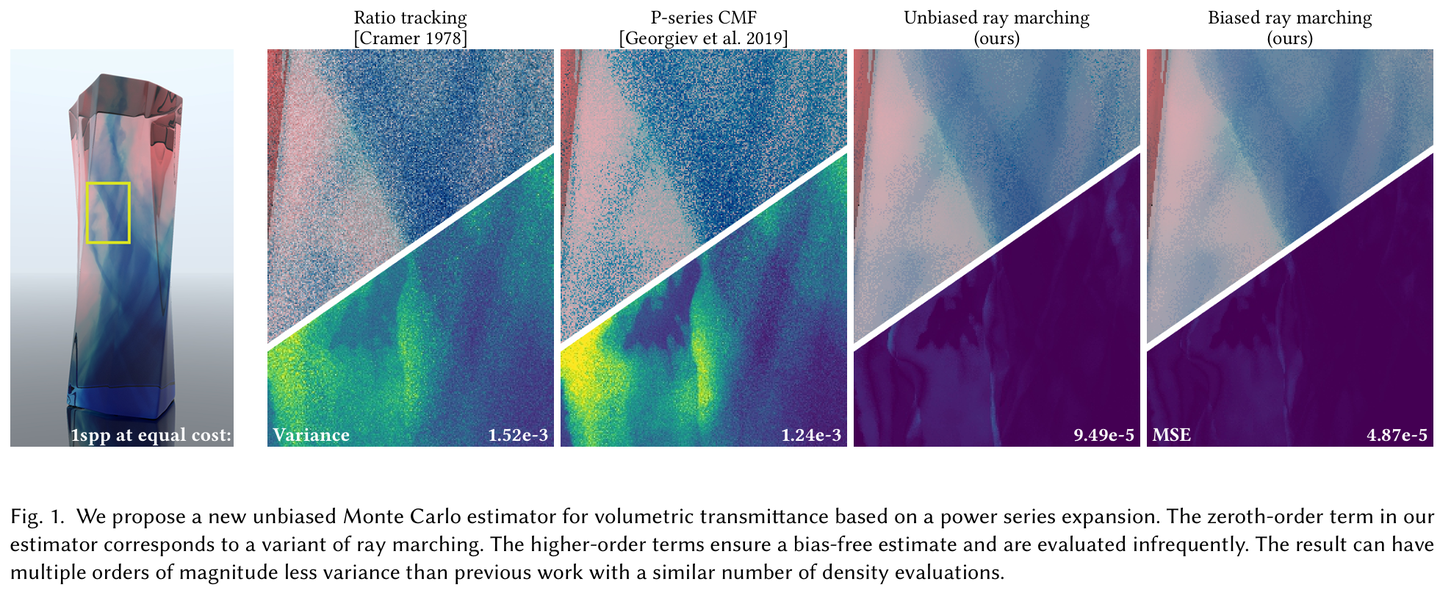
Main References

For the convenience of readers, the references are listed first; the main papers I read include:

1. Residual ratio tracking for estimating attenuation in participating media, ToG 2014
2. Monte Carlo Methods for Volumetric Light Transport Simulation, CGF 2018
3. Integral formulations of volumetric transmittance, ToG 2019
4. Direct Transmittance Estimation in Heterogeneous Participating Media Using Approximated Taylor Expansions, TVCG 2020
5. An unbiased ray-marching transmittance estimator, ToG 2021

It seems there has been no direct follow-up work after NVIDIA’s ToG 2021 paper. Other papers I read that are not in the rendering field are listed in the references. As reminded by a senior colleague, the volumetric rendering described in this article uses the classical participating media assumption; starting from ToG 2018, some papers began discussing media that do not satisfy exponential attenuation. Therefore, for rigor, the title includes the qualifier “Exponential Media.”

Notations

Since different volumetric rendering materials use different notation, \(\mu\) and \(\sigma\) are used interchangeably in this article, but within the same formula the notation is consistent. Specifically:

• \(\bar\mu\) and \(\sigma_{maj}\) are consistent, denoting an upper bound (majorant) of extinction;
• \(\mu\) and \(\sigma_t\) are consistent, denoting extinction;
• \(\mu_n\) and \(\sigma_n\) are consistent, denoting \(\sigma_{maj}-\sigma_t\).

Motivation

First, a brief review of the volumetric rendering pipeline, followed by an introduction to why Transmittance Estimation is needed. Those familiar can skip this section.

Volumetric Rendering Equation

We know the volumetric rendering equation (the sign of \(w\) depends on notation conventions; here we directly use PBRT’s):

That is, the incident radiance considers:

• \(T_r(p_s\rightarrow p)L_o(p_s,-w)\): the radiance reaching a non-participating medium point (e.g., a surface) \(p_s\), multiplied by the attenuation from traversing the medium;
• \(\int_0^{t_s} T_r(p'\rightarrow p)\sigma_t(p',w)L_s(p',-w)\mathrm dt\): the radiance contributed at each position along the current light path.

Where:

• \[L_s(p,w)=\frac{\sigma_a(p,w) L_e(p,w)+\sigma_s(p,w)\int_{S^2}\phi(p,w_i,w)L_i(p,w_i)\mathrm dw_i}{\sigma_t(p,w)}\]

  represents the emission at each position, plus radiance scattered from all directions (weighted by the phase function \(\phi\), analogous to the BSDF term for surfaces); dividing by \(\sigma_t=\sigma_a+\sigma_s\) keeps the dimensions consistent with radiance.

• \[T_r(p\rightarrow p')=e^{-\int_0^d\sigma_t(p+tw,w)\mathrm dt},\text{where }\ d=\|p-p'\|_2\]

  This term is called Transmittance, describing the energy attenuation of light traveling through a medium; we often refer to \(\int_0^d\sigma_t(p+tw,w)\mathrm dt\) as the optical thickness/depth, denoted by \(\tau\).

The above formulas are derived theoretically from the differential-integral equation of volumetric rendering via ordinary differential equations. Different approaches are used in offline and real-time rendering to estimate \(L_i\).

We Need to Estimate Transmittance!

In offline rendering, to ensure unbiasedness, Monte Carlo (MC) estimation is typically used. A classic approach starts with Russian Roulette (RR):

where \(u\in U[0,1],q\in(0,1)\); the first term is chosen with probability \(q\), and the second with probability \(1-q\), then \(E[\hat L]\) equals the original expression. Note that the second expression is still an integral, so another MC step is needed:

Thus Transmittance must always be estimated; in fact, since \(L_s\) also contains an integral, further MC steps are required.

In real-time rendering, for rendering speed, a biased Ray marching approach is typically used, estimating via Riemann sums:

Again, Transmittance estimation is required.

Note:

1. In offline rendering, there are ways to cleverly bypass the direct computation of Transmittance, but they fix the sampling strategy; these are given in the Appendix.
2. Real-time rendering can also use offline rendering methods, e.g., UE provides both PathTracing.hlsl and RayMarching.hlsl for sky rendering.

Back to Basics: Poisson Point Process

Before introducing how to estimate transmittance, let’s review some probability and statistics knowledge.

Poisson Distribution

Among discrete random variables, there are three very common distributions:

• Bernoulli Distribution: A single trial with only two outcomes (0 and 1), with success probability determined by a single parameter \(p\); its PMF is \(P(X=1)=p, P(X=0)=1-p\); \(E(X)=p\).
  • Flipping a coin once, with equal probability for heads and tails, so \(p=0.5\).
• Binomial Distribution: Performing \(n\) independent Bernoulli trials, the PMF for the number of successes \(k\) is: \(P(X=k)=C_n^k p^k (1-p)^{n-k}\); \(E(X)=np\).
  • The probability of getting \(k\) heads in \(n\) coin flips.
• Poisson Distribution: The binomial distribution can only describe discrete trials. However, in some cases, events can occur at any moment within a unit of time, but the success probability is extremely small, satisfying only \(\lim_{n\rightarrow \infty}np=\lambda\). In these infinitely many trials, the probability of \(k\) successes is \(P(X=k)=\lambda^k e^{-\lambda}/k!\); \(E(X)=\lambda\).
  • For example, in a 90-minute soccer match, goals can happen at any moment, but we only know the average number of goals is 2.5; then we can use a Poisson distribution with \(\lambda=2.5\) to calculate the probability of the actual number of goals.

The Poisson distribution essentially describes a process where:

• Events at each moment are independent, with uniform success probability; past events do not affect the probability of future events occurring;
• Within a given time interval, an average of \(\lambda\) successful events occur.

Properties of Poisson Distribution

The Poisson distribution has several remarkable properties:

1. The time interval between two successive events follows an exponential distribution \(Exp(\lambda)\).

   Proof: Since the success probability is uniform, assume the next event occurs at time \(T\); we can instead compute the probability that no event has occurred by time \(T\): \(P(X=0)=e^{-\lambda T}\) (this is because the average rate per unit time is \(\lambda\), so over time \(T\) the average is \(\lambda T\)).

   Therefore, the CDF is \(P(t\leq T)=1-e^{-\lambda T}\), and differentiating gives the PDF \(p(t)=\lambda e^{-\lambda t}\).

2. If the time intervals between events follow an exponential distribution, then the number of events follows a Poisson distribution.

   Proof: \(P(X=0)\) is easily shown as above; then by mathematical induction, assuming \(P(X=k)\) satisfies the Poisson distribution:

   \[\begin{aligned} P(X=k+1) & =\int_0^t P\left(\text {First arrival at } t_1<t \text { and exactly } k \text { arrivals between } t_1 \text { and } t\right) \mathrm d t_1 \\ & =\int_0^t \lambda \exp \left(-\lambda t_1\right)\left(\lambda\left(t-t_1\right)\right)^k \frac{\exp \left(-\lambda\left(t-t_1\right)\right)}{k!} d t_1 \\ & =\frac{\lambda^{k+1} \exp (-\lambda t)}{k!} \int_0^t\left(t-t_1\right)^k d t_1 \\ & =\frac{(\lambda t)^{k+1} \exp (-\lambda t)}{(k+1)!} \end{aligned}\]

3. If it is known that one event occurred in the current time interval, then the event’s occurrence time is uniformly distributed. Formally, \(P(x)=P(X\leq x\mid N_t=1)=x/t\) \(\Rightarrow p(x)=1/t\).

   Proof:

   \[\begin{aligned} P\left(S_1 \leq\right. \left.x \mid N_t=1\right)&=\frac{P\left(S_1 \leq x, N_t=1\right)}{P\left(N_t=1\right)} \\ & =\frac{P\left(N_x=1, N_t-N_x=0\right)}{P\left(N_t=1\right)} \\ & = \frac{P\left(N_x=1\right) P\left(N_t-N_x=0\right)}{P\left(N_t=1\right)} \\ & =\frac{P\left(N_x=1\right) P\left(N_{t-x}=0\right)}{P\left(N_t=1\right)} \\ & =\frac{\alpha x e^{-\alpha x} \cdot e^{-\alpha(t-x)}}{\alpha t e^{-\alpha t}}=\frac{x}{t} \end{aligned}\]

   Generalized conclusion: If \(N\) events occurred in the current interval, then the \(N\) events are i.i.d. \(U[0, t]\). See proof on StackExchange.

Non-Stationary Poisson Distribution

The Poisson distribution we considered above is a special case where the success probability is uniform. But what if the success probability is not uniform? Let’s first consider the simplest case: a two-segment piecewise uniform Poisson distribution.

Suppose the first segment satisfies \(N\sim \text{Po}(\lambda_1)\), and the second segment satisfies \(N\sim \text{Po}(\lambda_2)\). Then the probability of \(n\) successful events in the entire interval is the sum over \(k\) and \(n-k\) events in the two segments:

By the binomial theorem:

Thus:

Therefore, overall, \(N\sim \text{Po}(\lambda_1+\lambda_2)\); however, since the probability changes in the middle, some properties are slightly degraded, e.g., the overall arrival time no longer follows an exponential distribution.

Poisson Point Process (PPP)

More generally, the event probability varies with time, satisfying only the following two properties:

• Events at each moment are independent; past events do not affect the probability of future events;
• At time \(t\), if the Poisson distribution is followed according to the current rate, the average number of successful events per unit time is \(\lambda(t)\).

We call this process a Poisson Point Process (PPP); the homogeneous Poisson distribution is a homogeneous PPP. We call \(\lambda(t)\) the intensity function or rate function.

From a calculus perspective, we can consider \(\lambda\) to be constant within each small \(\delta\), forming several piecewise Poisson distributions. It follows that: for any interval \(t_0\sim t_1\), the number of events satisfies \(N\sim \text{Po}(\int_{t_0}^{t_1}\lambda(t)\mathrm dt)\), with expected value \(E(N)=\int_{t_0}^{t_1}\lambda(t)\mathrm dt\). In particular, \(P(N=0)=e^{-\int_{t_0}^{t_1}\lambda(t)\mathrm dt}\).

In mathematics, the definition of PPP is more relaxed, controlled only through limits. I cannot understand how to prove the above properties of PPP from the relaxed definition; I only managed to prove \(P(N=0)\) through bounding and the squeeze theorem. Since this does not affect our main topic, interested readers can see the Appendix.

So how do we sample a sequence of points from a PPP given \(\lambda(t)\)? We could use inverse CMF, but computing the integral is too complicated, so the most common method is called Thinning (see other references [Pausupathy2011]):

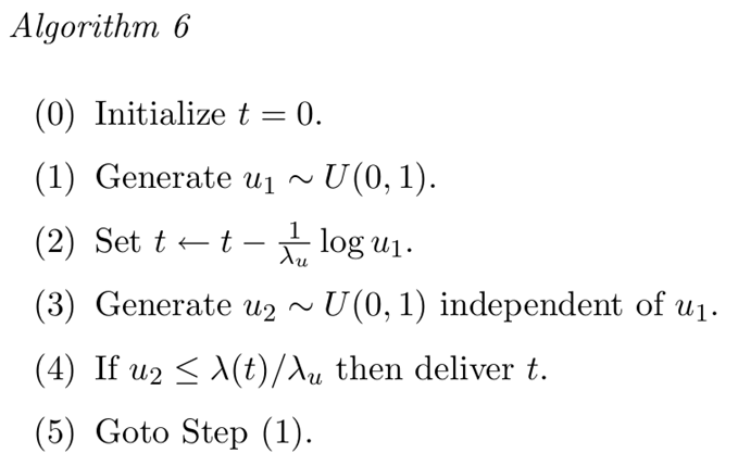
Simply put, it applies the principle of rejection sampling. We first fill the PPP’s \(\lambda(t)\) up to an upper bound \(\lambda_u\), forming a pure Poisson distribution. For this Poisson distribution, we can use the exponential distribution to sample a point sequence. However, since we have overestimated the event probability, we must reject some points; the rejection is done by a Bernoulli distribution with probability \(\lambda(t)/\lambda_u\) at each point. For a rigorous proof, see other references [Lewis & Shedler 1978].

Current Estimators

Our core focus is \(T_r(p\rightarrow p')=e^{-\int_0^d\sigma_t(p+tw,w)\mathrm dt}\); note that there is still an integral, which can also be estimated via biased Riemann sum or unbiased MC.

Ray Marching Estimator

Similar to the estimation of the volumetric rendering equation, we can use ray marching:

The most naive approach is to ray-march \(N\) intervals in the volumetric rendering equation, and for each interval estimate the transmittance with \(M\) sub-intervals, resulting in \(O(NM)\) complexity. However, the sampling points for Transmittance Estimation can reuse those from the volumetric rendering equation, allowing estimation of the entire equation at \(O(N)\) speed. In this case:

From the current sampling point to the next, we only need \(\text{Tr}_{i}=\text{Tr}_{i-1}\cdot e^{-\sigma_t(p_i',w)\delta t_{i-1}}\), without needing to compute \(M\) times for each point. Using a fixed step size is very common, and the pseudocode is as follows:

// N is the number of ray marching intervals, offset is an arbitrary offset to the interval, not necessarily starting at the intersection.
float RayMarching(Volume volume, float3 pos, float3 dir,
                  float tMax, int N, float offset = 0.5f)
{
    float stepSize = tMax / N;
    float t = offset * stepSize;
    pos += dir * offset * stepSize;
    
    // Transmittance due to the initial offset; if no offset, it's 1.
    float transmittance = exp(-volume.SampleExtinction(pos) * offset);
    float radiance = 0; // In real-time rendering, directly RGB; the sampled result is also RGB.
    for (int i = 0; i < N; i++)
    {
        float newRadiance = GetRadiance(volume, pos, dir); // We assume this computes sigma_t * L_s
        radiance += newRadiance * stepSize * transmittance;
        
        // Reuse the current sampling point to update the transmittance for the next segment
        float extinction = volume.SampleExtinction(pos);
        transmittance *= exp(-extinction * stepSize);
        t += stepSize;
        pos += dir * stepSize;
    }
    
    return radiance;
}

Of course, there are more complex implementations that do not use a fixed step size, but the Riemann sum principle remains unchanged.

Pitfalls of Stochastic Estimators

Before introducing the estimation of Transmittance in offline rendering, we need to clarify a concept and resolve a common misconception. When we see an integral, we might naturally use MC for the following estimation:

Here we have abbreviated: \(\sigma_t(X)\) denotes \(\sigma_t(p+xw,w), x\sim p(X)\). After estimating the optical depth, simply computing \(e^{-\hat\tau}\) gives us an estimate of transmittance — so easy!

Well, not that easy. In fact, we are making the assumption:

In our case, this is \(e^{-E(X)}=E(e^{-X})\). Let’s first consider a discrete random variable with \(N\) possible values \(x_1,\cdots ,x_N\):

These clearly don’t look equal! Those familiar with inequalities should immediately recognize Jensen’s Inequality:

Clearly \(e^{-x}\) is convex, so this estimation method is biased (Jensen’s gap) and will always overestimate. For continuous \(X\), the same conclusion can be derived through the measure space of probability.

On the other hand, some might say: since \(\sum_{i=1}^N e^{-\hat\tau_i}/N\) doesn’t work, let’s first estimate the optical depth more accurately, i.e., set \(\tau_0=\sum_{i=1}^N \hat\tau_i/N\), and then compute \(e^{-\tau_0}\). This should be unbiased, right? Unfortunately, still no. We’ve only replaced the estimator inside the exponent with a more accurate one, then performed a single sample as the estimation result; Jensen’s Inequality still gives \(E[e^{-\bar X}]\geq e^{-E[\bar X]}\). For example, let \(X_i\sim N(\mu,\sigma)\), then \(E[e^{-\bar X}]=e^{-\mu+\frac{\sigma^2}{2N}}\), which is not unbiased, only at most consistent.

In summary, estimating optical depth and then exponentiating will always overestimate transmittance and is not an unbiased estimator.

Of course, if you are doing real-time rendering and don’t care about bias, it doesn’t matter.

Delta-Tracking Estimator

Observe the formulas for PPP \(P(N=0)\) and Transmittance:

Since the extinction coefficient \(\sigma_t\) is always non-negative, transmittance is the probability that a PPP with rate function \(\sigma_t(t)\) has zero events. Therefore, if we sample a sequence following the Thinning procedure, only an empty sequence corresponds to \(N=0\); by performing enough Thinning samples and counting the frequency of \(N=0\), we can estimate the probability. Of course, since sampling the first successful event already indicates failure, we can terminate early, leading to the Delta Tracking algorithm:

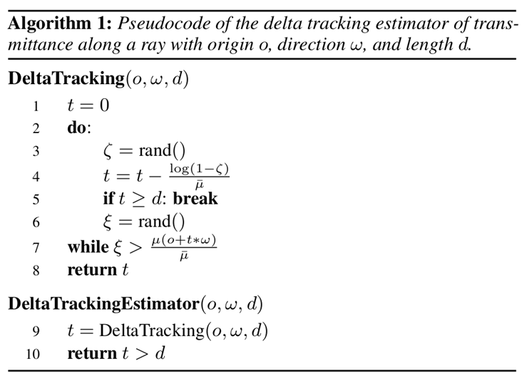
Different papers use different notation; here \(\mu\) represents \(\sigma_t\), and \(\bar \mu\) represents the upper bound for Thinning. We will also use \(\mu\) and \(\sigma_t\) interchangeably later.

Here, \(t\geq d\) means the PPP has left the current time interval, so no events were sampled; \(\xi > \mu/\bar\mu\) represents the rejection sampling process. For Delta-Tracking Estimation, we can also use finer-grained upper bounds (piecewise-constant / piecewise-linear / piecewise-polynomial, with corresponding changes to the sampling method) to prevent the upper bound from being too large, which would generate more sample points and require more rejection computations.

Ratio-Tracking Estimator

Although Thinning nicely solves the bias problem, this simulation-style sampling seems inefficient. Is it possible to use the entire sampled sequence for estimation? Let’s first observe the Delta-Tracking algorithm; it actually resembles the RR process in ray tracing. At first glance, it might not look similar, so let’s rewrite it in recursive form:

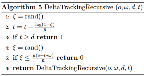
Line 2 resembles finding an intersection, line 3 resembles reaching the light source, and lines 4-5 are like RR, continuing to the next hop with some probability (line 6) or stopping. That is, the Delta-Tracking algorithm is equivalent to the following estimator transformation:

Thus \(E[\hat T_r(a,b)]=E[(1-\mu(x)/\bar\mu)\cdot \hat T_r(x,b)]\), with the sampling of \(x\) being exponential sampling. Therefore, to estimate \((a,b)\), first sample \(x_1\), then estimate \((x_1,b)\); to estimate \((x_1,b)\), sample \(x_2\), and so on (this is the same as converting multi-bounce ray tracing recursion into a loop). This yields the Ratio-Tracking Estimator:

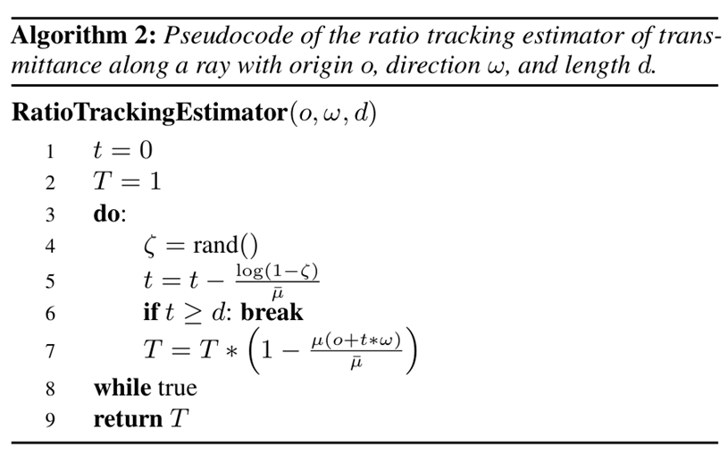
Line 7 continuously transfers the result to a new estimator until exiting the volume (at which point transmittance is 1).

Residual Ratio-Tracking Estimator

Notice that in PPP we need to fill up to an upper bound, and the larger the filled \(\lambda\), the more samples the exponential distribution requires, increasing the complexity of a single estimation. As mentioned earlier, this can be partially addressed by using a tighter upper bound. But if \(\lambda(t)\) is consistently large, the lower bound itself is already large, and a tighter upper bound doesn’t help much. In this case, we can uniformly remove part of the lower bound:

We can treat \(\sigma_t-\sigma_c\) as the new extinction for estimation, yielding the Residual Ratio-Tracking Estimator algorithm:

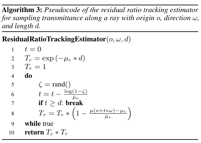
where \(\bar\mu_r\) is the new upper bound \(\bar\mu-\mu_c\).

In particular, this “removal” process is a classic method for variance reduction in MC — control variate. Simply put, estimating \(X\) might not be very good, but subtracting another random variable \(Y-E[Y]\) can make it easier to estimate, keeping the expectation unchanged while reducing variance. In volumetric rendering, we always see subtraction of a uniform constant, so we won’t elaborate on the theory of control variates.

Furthermore, the original paper provides an intuitive explanation for this removal, suggesting that \(\sigma_c\leq \sigma_t\) is not required. However, for the PPP interpretation to hold, the rate function must be non-negative everywhere. A rigorous proof of the original paper’s method can be given through the subsequent Estimator theory.

Power-Series Estimator: Include All Above!

Note that although estimating \(X\) cannot be generally used to estimate \(f(X)\), polynomial functions \(f\) are special. Of course, functions like \(x^2\) still have a Jensen gap when estimated with a single sample, but independent random variables have a very special property:

Therefore, suppose we want to estimate \(a^2\), and we can only obtain \(E[X]=a\). Then we can sample twice and multiply: \(E[X_1X_2]=E[X_1]E[X_2]=a^2\). But we need to estimate \(e^x\) — how can we convert it into a polynomial?

That’s right, the infinite power series comes to the rescue! We know (easily obtained from Taylor expansion as well):

We just need to estimate each term and sum them up; by the additivity of expectation, we obtain an estimate of \(e^x\):

However, we clearly cannot compute every term of an infinite series, so different methods yield different Estimators.

Single-term Estimator

Lu Xun once said: I seem to have contracted some disease — whenever I see infinite space, I think of MC.

We can still apply MC to the series. Note that for a general function \(f(k)\):

where \(\kappa\) is a discrete random variable satisfying \(p(\kappa)\), with non-zero probability for each value. We only need to draw one index and estimate that term:

In Transmittance estimation, since \(x\) is an integral, we can continue with MC. For example, to estimate \(-\tau=-\int_0^d\sigma_t(p+tw,w)\mathrm dt\):

Since the signs of the series terms keep alternating due to the negative part, causing numerical instability, we can instead estimate \(\tau_n\):

This gives:

Thus:

In particular, we can prove that all the previous stochastic estimators are single-term estimators:

• Ratio-Tracking Estimator: Note that the sampling of \(t\) in the algorithm is exponential sampling, meaning the number of estimates follows a Poisson distribution \(k\sim\text{Po}(\bar\tau)\), and the sampling follows \(\text{Exp}(\sigma_{maj})\), i.e.:

  \[p_1(k)=\bar\tau^k e^{-\bar\tau}/k!, p_2(x)=\sigma_{maj}/\bar\tau\]

  Substituting:

  \[\frac{e^{-\bar\tau}}{k!\tau^k e^{-\bar\tau}/k!}\cdot\prod_{i=1}^k \frac{\sigma_n(X_i)}{\sigma_{maj}/\bar\tau}=\prod_{i=1}^k\frac{\sigma_n(X_i)}{\sigma_{maj}},\text{where }X_i\sim p_2(x)\]

  This is consistent with the estimation method of the Ratio-Tracking Estimator.

• Delta-Tracking Estimator: This can be seen as also performing \(k\) events, but the algorithm terminates early at the \(i\)-th event (each event performs a Bernoulli trial with probability \(\sigma_n/\sigma_{maj}\) to decide whether to terminate). Overall, it is equivalent to \(\hat T=1\) with probability \(\tau_n\), and \(\hat T=0\) otherwise.

• Residual Ratio-Tracking Estimator: Similar to the Ratio-Tracking Estimator, but with the lower bound removed: \(k\sim\text{Po}(\bar\tau-\tau_c)\), \(x\sim\text{Exp}\left((\sigma_{maj}-\sigma_c)/(\bar\tau-\tau_c)\right)\).

  From this perspective, we only need to ensure \(\bar\mu_r\geq 0\) for sampling \(k\) to work; it is not necessary that \(\sigma_c\leq \sigma_t\), since from the series perspective we no longer rely on the PPP requirement that the rate must be non-negative — a negative value just introduces oscillation.

The TVCG 2020 paper also applied other distributions from this perspective, such as the geometric distribution.

Truncated Estimator

As we can see, the single-term estimator estimates \(k\) samples of \(X\) each time, but only uses a single \(E[X]^k\) term, which is somewhat wasteful. The additivity of expectation does not require independence, so we could compute all the powers at once. This gives rise to the Truncated Power-series Estimator:

That is, \(P_k\) is (1 minus the cumulative probability up to \(k-1\)). In practice, we just sample one \(n\), then sample \(X_i\) and compute the terms above.

We now prove the correctness of the above estimator. First, we prove the following identity:

More abstractly, we can prove:

Let’s first consider the finite case for an intuitive geometric understanding:

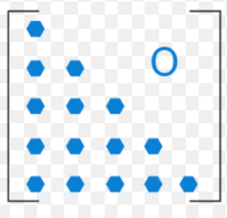
Where \(a_{ij}\) are elements of a lower triangular matrix. The LHS sums over each row (outer sum selects the row), and the RHS sums over each column (outer sum selects the column); both compute the sum of all matrix elements, so the two are equal. Intuitively, letting \(n\rightarrow\infty\) proves our identity. Let \(h(n)=p(n), g(k)=P_k\), then:

Since \(P_k=\sum_{m=k}^{\infty}p(m)\), the numerator and denominator cancel:

Great, another opportunity for MC! In our scenario, \(f(k)=x^k/k!\), and \(x\) must be estimated by \(X_i\), so:

QED.

Those familiar with mathematical analysis will notice that the order of summation in infinite series cannot be arbitrarily swapped, and our proof above is not rigorous. However, if the series converges absolutely, then any rearrangement converges to the same value, and the above identity holds (the more general integral exchange is Fubini’s theorem in real analysis). In our scenario, the series converges absolutely to \(e^{\lvert x\rvert}\), so it is still correct.

Recursive Estimator

We can also write \(e^x\) in recursive form. First:

Define \(a_{ij}=x/j\) (so each column has the same element). Again, let’s visualize:

The expression above corresponds to multiplying each row and then summing. Suppose we already have the triangle \(M_{j+1}\) at the bottom-right. Extending one column to the left is essentially the current triangle multiplied by \(x/j\), plus the top-left element:

Expanding \(M_1\) layer by layer:

Adding back the initial 1 and substituting \(x=-\tau\):

Thus we can use the following estimator:

This is very similar to ray tracing’s continuous search for the next hit, so RR can be applied. More generally, we can also insert a \(\bar\tau\):

Combining \(e^{-\bar\tau}\hat T_j\) as the new \(\hat T_j\):

Following the original paper’s formula, this is just inserting \(\bar\tau\); in fact, using the top-level formula to directly estimate \(e^{\tau_n}\) and then multiplying by \(e^{-\bar\tau}\) works just as well.

Applying RR:

Substituting \(\hat\tau_n=\sigma_n(X)/p(X)\), we finally obtain:

Detailed Tricks

The following content is not directly related to the principle of the Estimators themselves, but rather how to choose certain parameters or optimize variance. So we list them in a separate section.

At least 99%!

Although stochastic estimators are unbiased, there is still noticeable noise with limited samples. Therefore, if we can determine the contribution of each term, we can first compute the bulk of the contribution from the series and then sample the remainder to maintain unbiasedness. Notice:

If we multiply both sides by \(e^{-x}\), we get \(1=\sum_{i=0}^\infty e^{-x}x^i/i!\). This reveals that the contribution of the \(k\)-th term of the series is consistent with \(P(N=k)\) of the Poisson distribution \(\text{Po}(x)\). Of course, when computing \(e^{\tau_n}\), we don’t know the true value of \(\tau_n\), but we can guarantee a lower bound on the contribution. For example, since \(\bar\tau\geq \tau_n\), if we use \(\text{Po}(\bar\tau)\) to estimate the contribution, the number of events will be overestimated and the CMF will grow more slowly, as shown below:

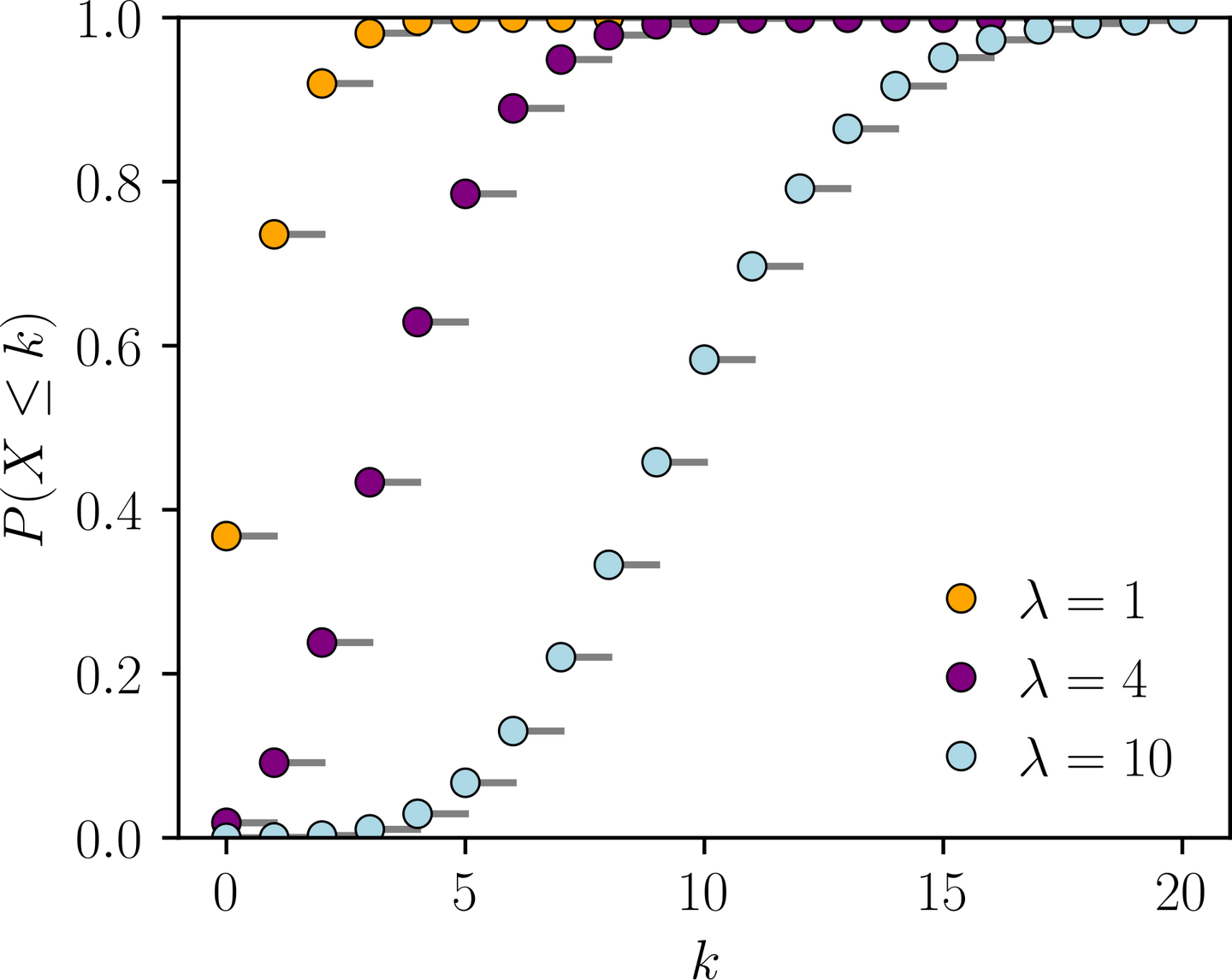
If we can guarantee that 99% of the contribution is reached under \(\text{Po}(\bar\tau)\), then we are assured that 99% of the contribution is also reached under \(\text{Po}(\tau_n)\).

In the Recursive Estimator, we can then use the following RR probability:

In the Truncated Estimator, we can also fix the first \(K\) terms (equivalent to setting \(P_k\equiv 1\) for those terms), and then determine the specific number of terms \(n\) via RR.

How to Choose Pivot?

Notice that the choice of \(\sigma_c\) determines estimation efficiency. We previously explained that \(\sigma_c\) can be chosen as a lower bound to reduce overhead; the subsequent series derivation further shows that it doesn’t have to be a lower bound — any value works. Ideally, if \(\tau_c=\tau\), there would be nothing to estimate, and variance would be zero. But \(\tau\) itself is unknown. So NVIDIA 2021 proposed sampling an additional sample \(X_{n+1}\), using \(\hat\tau\) as the pivot (cannot use \(X_1,\cdots X_n\), as that would violate the independence of estimation and introduce bias); rotate through each sample as the pivot, estimate \(n+1\) times, and average the results.

Maximize Utilization of Estimation

In the Truncated Power-series Estimator, although we improve sample utilization by estimating the first \(K\) terms, note that the first term only uses \(X_1\), the second term only uses \(X_1\cdot X_2\), and so on. We could instead leverage all samples: the first term uses \(\sum X_i/N\), the second term uses \(\sum X_iX_j/C_{n}^2\), and so on (this method is called U-statistics in NVIDIA 2021).

Of course, computing all combinations is too complex, but if we use all terms, the following \(O(N^2)\) recursive algorithm can be employed:

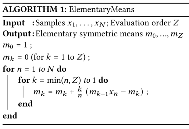
“Unbiased Ray Marching”

Based on the above algorithms, NVIDIA 2021 proposed the so-called Unbiased ray marching estimator:

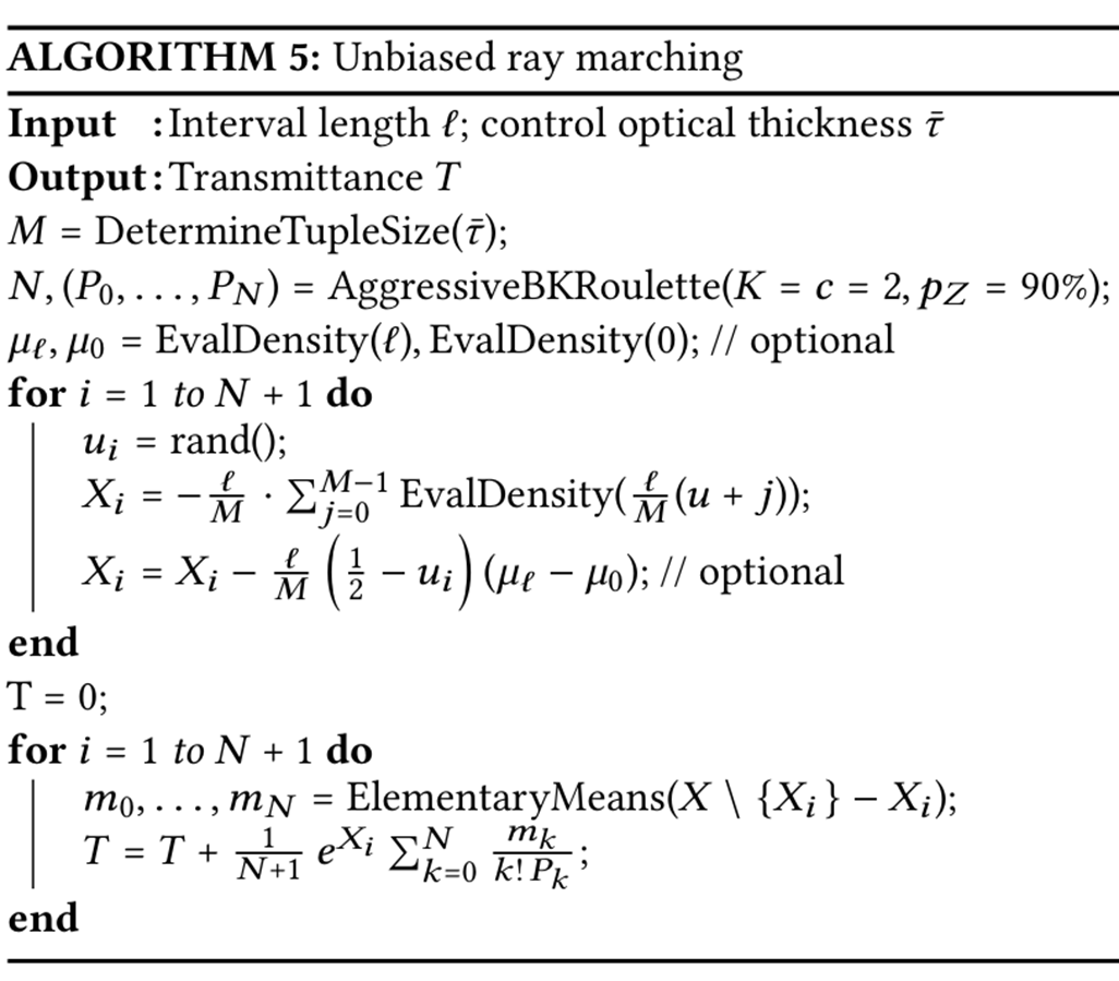
Brief explanation:

1. Our previous \(X_i=\sigma_n(X)/p(X)\) only sampled once as an MC estimate, but we can sample multiple times and average to obtain \(X_i\); here \(M\) determines how many samples to take. DetermineTupleSize is an empirical formula:

   • First, based on Truncated Series CMF > 0.99, determine the total number of terms to estimate (the original paper gives a grid-searched approximate formula \(N_{CMF}=\) \(\lceil\sqrt[3]{(0.015+\bar{\tau})(0.65+\bar{\tau})(60.3+\bar{\tau})}\rceil\)), considering that at least this many samples are needed for good results;
   • Then simulate Roulette to compute the expected order \(E[N]\).
   • Finally, \(N_{CMF}/E[N]\) gives the number of samples per order to average.

2. AggregateBKRoulette is our previous process of Roulette over orders, but the formula is slightly generalized:

   \[e^x=\sum_{k=0}^K \frac{x^k}{k!}+\frac{c}{K+1}\left(\frac{x^{K+1}}{c K!}+\frac{c}{K+2}\left(\frac{x^{K+2}}{c^2 K!}+\ldots\right.\right.\]

   Essentially unchanged; although the original paper discusses a lot of theory, in practice they simply set \(K=c=2\), so there’s not much need to elaborate further. In particular, to reduce overhead, there is a probability \(p_Z\) of computing no terms at all.

3. The middle part of computing \(X_i\) looks like ray marching, but actually only the sampling points are equally spaced; the first point is sampled randomly (imagine partitioning the integral and MC-sampling each segment; since expectation is additive and independence is not required, the same \(u\) can be used for all segments). Of course, this kind of sampling doesn’t look great, so other methods are needed to reduce noise.

4. The two optional lines reduce the error caused by equiv-distance sampling. The paper mentions CP-rotation, pointing out that this type of sampling is equivalent to a cyclic shift of the function, causing discontinuity at the two endpoints and increasing error. The paper proposes density reshuffling, with the formula:

   \[\mu^{\star}(s):=\mu(s)+\left(\frac{1}{2}-\frac{s}{\ell}\right)(\mu(\ell)-\mu(0)) .\]

   This is an affine transformation that makes the two endpoints equal under this transformation while preserving the integral value of \(\mu^\star\) to be consistent with \(\mu\).

5. Finally, ElementaryMeans computes the average over all permutations, cycling through each \(X_i\) as the pivot, and uses the Truncated Estimator to compute the Transmittance estimate.

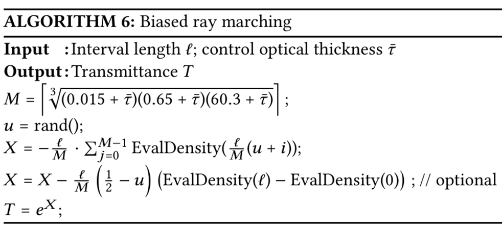
The paper also gives a faster but biased algorithm, which is essentially the \(e^{E[X]}\) approach we discussed earlier, but with some of the above methods to reduce error:

Appendix

Additional Results

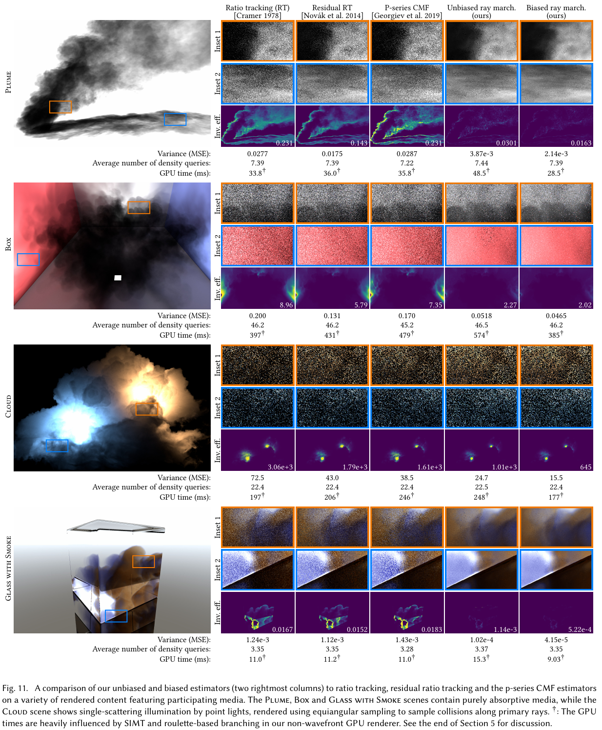
P-series CMF refers to Recursive Estimator + CMF at least 99%, and the last two columns use all the tricks from NVIDIA 2021.

Skip Transmittance Estimation

We mentioned earlier that offline rendering can bypass Transmittance Estimation. Consider the following expression again:

Assume the volume is homogeneous, with \(\sigma_t\) constant, so \(T_r=e^{-\sigma_t d}\). Then setting \(q=e^{-\sigma_td}\) cancels \(T_r\) in the first term. For the second term, note that \(1-e^{-\sigma_t d}\) is exactly \(\text{Pr}(t\in [0,d])\) for \(\text{Exp}(\sigma_t)\), so we can directly sample \(t\sim \text{Exp}(\sigma_t)\), choosing the first term when \(t\in [d,+\infty)\).

Also note that the integral in the second term requires an MC estimate over \([0,d]\). If we use the \(t\) sampled above, the corresponding PDF for MC is the normalized \(\text{Exp}(\sigma_t)\), i.e., \(\sigma_t e^{-\sigma_tt}/(1-T_s)=\sigma_t T_r(p+wt,p)/(1-T_s)\). Thus the second term can be written as:

Canceling terms yields:

Of course, this assumes a homogeneous volume. If \(\sigma_t\) varies, we can use a Thinning-like approach to first fill up to a homogeneous bound, then “remove” the excess \(\sigma_n\):

A rigorous proof that the computed radiance is equivalent to the original radiance still requires ordinary differential equations, which are omitted here. But we can follow the estimation method above, treating the extra \(\sigma_n\) as a possible light path:

Then RR over the three terms of \(L_n\):

This avoids all Transmittance Estimation. The physical intuition of the above equations is that a light beam may encounter three types of events:

• Self-emitting particles that add radiance;
• Scattering events, where light scatters into a different direction (the new light path sampled by the MC second term);
• Null particle events, which are the imaginary particles added by the \(\sigma_{maj}\) fill — these events do not actually occur, and the light path continues in the current direction.

Mathematical Formulation of PPP

Many sources define PPP formally as:

I can’t fully understand how to prove that any segment satisfies \(N\sim \text{Po}(\int_{t_0}^{t_1}\lambda(t)\mathrm dt)\). I only managed to prove \(P(N=0)\):

Starting from the definition of the limit, we can define the corresponding sequence and take the log of both sides:

Note that:

Hence:

Taking the exponential of both sides and applying the squeeze theorem gives \(P(N=0)=e^{-\int_t^{t+T} \lambda(t) \mathrm{d} t}\). QED.

Intuition suggests mathematical induction should still work, but since it’s not related to volumetric rendering, I didn’t pursue it further.

Other References

For the basic theory of volumetric rendering, see PBRT.

Other references I actually read that are unrelated to volumetric rendering:

1. Particle Filters for Partially Observed Diffusions, Fearnhead et.al.
2. An Introduction to the Theory of Point Processes: Volume I: Elementary Theory and Methods, 2nd ed., D.J. Daley & D. Vere-Jones.
3. Generating Nonhomogeneous Poisson Processes, Pasupathy.
4. Simulation of nonhomogeneous poisson processes by thinning, Lewis & Shedler.